
RAG Systems: Optimizing Embedding Storage Costs
How to cut RAG embedding storage costs by tuning dimensions, chunking, indexes, and lifecycle controls while protecting retrieval quality.

Embedding storage can stay cheap at small scale, then get expensive fast when chunk counts and RAM-heavy indexes grow. If I want to control spend in a RAG system, I need to focus on four levers right away: embedding size, chunk count, index overhead, and data cleanup.
Here’s the short version:
- Higher dimensions cost more per chunk. A 3,072-dimension vector uses 8x the raw storage of a 384-dimension vector at float32.
- More chunks means more vectors. If I double chunk count, I double raw vector storage.
- Indexes often cost more than raw vectors. In many setups, total footprint lands around 1.5x to 3x the raw vector size.
- Compression helps, but quality can drop. FP16, INT8, INT4, PQ, and binary methods can cut storage, but I still need to test recall, ranking quality, and answer accuracy.
- Dimension cuts save more space, but come with more work. Re-indexing, validation, and model changes can add $12,000 to $18,000 in one-time engineering cost.
- Storage control is not just compression. Delete-before-insert, delta sync, chunk-size tuning, and compact persistence formats all help keep growth in check.
- Finetuning vs. RAG comparisons show that RAG can still cut inference spend by 60% to 80% versus sending large context windows on every request, so storage tuning helps protect those savings.
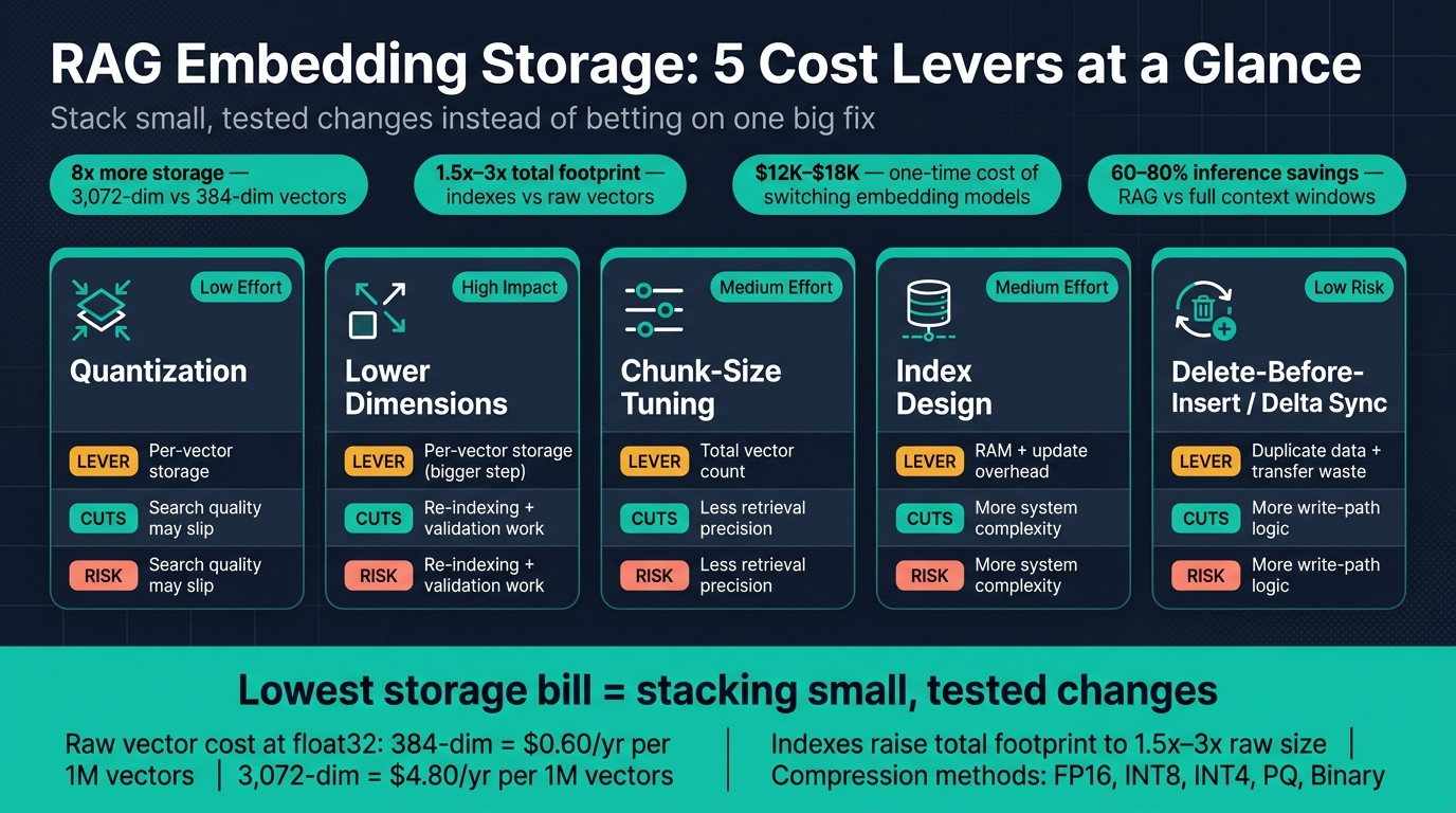
RAG Embedding Storage Cost Levers: What to Cut and What It Costs You
Quick comparison
| Lever | What it cuts | Main cost/risk |
|---|---|---|
| Quantization | Per-vector storage | Search quality may slip |
| Lower dimensions | Per-vector storage at a bigger step | Re-indexing and validation work |
| Chunk-size tuning | Total vector count | Less retrieval precision |
| Index design | RAM and update overhead | More system complexity |
| Delete-before-insert / delta sync | Duplicate data and transfer waste | More write-path logic |
If I had to sum it up in one line, it would be this: the lowest storage bill usually comes from stacking small, tested changes instead of betting on one big fix.
sbb-itb-f123e37
Baseline Storage in Production RAG Systems
Baseline storage comes from three variables: chunk count, vector dimension, and numeric precision. For organizations scaling these systems, NAITIVE AI Consulting provides the architectural expertise needed to manage production overhead. This gives you the starting storage cost before any compression enters the picture.
How Chunking, Vector Count, and Dimensions Shape Storage
Dimension count is the clearest driver of per-vector size. At float32 precision, each value uses 4 bytes. So a 384-dimension vector takes 1,536 bytes, while a 3,072-dimension vector - like the ones from OpenAI's text-embedding-3-large - takes 12,288 bytes. That's 8× more storage per chunk.
| Dimension Count | Per-Vector Size | Storage per 1M Vectors | Est. Annual Cost ($400/TB) |
|---|---|---|---|
| 384 | 1,536 bytes | ~1.54 GB | ~$0.60 |
| 768 | 3,072 bytes | ~3.07 GB | ~$1.20 |
| 1,536 | 6,144 bytes | ~6.14 GB | ~$2.40 |
| 3,072 | 12,288 bytes | ~12.29 GB | ~$4.80 |
Raw vectors only; indexes usually raise total footprint to 1.5× to 3×.
Chunk count scales storage in a straight line. Double the chunks, and you double the raw vector footprint. Simple as that. That raw footprint is the reference point for the compression results that follow.
Index Structure and Memory Overhead
Raw vector size is only the starting point. In production, memory-resident indexes often drive more of the bill than the vectors themselves. HNSW, for example, is often kept in RAM to support low-latency search, and that overhead can be larger than the raw vector footprint.
Next: which compression methods shrink this baseline without hurting retrieval quality.
What Recent Research Shows on Compression and Dimensionality Reduction
Once you know your baseline storage cost, the next step is figuring out how much you can shrink it - and what you give up in the process. Recent research points to quantization and dimensionality reduction as the two main ways to cut embedding storage.
Quantization Results: float8, int8, PQ, and Binary
Recent work looks at float8, FP16, INT8, INT4, product quantization (PQ), and binary embeddings as compression options for production RAG systems. Methods like FP16, INT8, and INT4 can cut storage and may also improve retrieval throughput.
That said, there’s no one-size-fits-all pick. A method that saves space on paper can still hurt search quality in practice. The safe move is to test each option against the metrics that matter most for your setup:
- recall
- ranking quality
- answer accuracy
Dimensionality Reduction Results and Order of Operations
If quantization still doesn’t cut storage enough, dimensionality reduction is the next lever. Dropping dimensions can save even more space, but it also brings extra work. In most cases, that means re-indexing and another round of validation.
Recent studies test how far embedding dimensions can fall before recall, ranking quality, or downstream answer accuracy starts to slip. They also look at which dimension targets give the best storage savings for the least quality loss. There’s a bigger issue here too: changing embedding models can force full retraining and a large round of benchmark re-validation, with model-switching costs reaching $12,000 to $18,000 in one-time engineering effort.
So embedding dimensionality isn’t just a storage tweak. It’s an architecture choice. Before locking in a target, weigh the space savings against the cost of re-indexing, retraining, and validation. That’s why storage design - not just model choice - sits at the center of the cost plan.
Storage Architecture and Data Lifecycle Controls
After compression, the next place to cut costs is storage layout and data lifecycle controls. If compression has already done most of the heavy lifting, the next step is to manage how data moves, where copies pile up, and when old data gets removed.
Index Choice and Update Path Design
The write path has a big effect on storage use. If updates trigger too much reindexing or sync work, storage and compute costs can creep up fast.
A simple way to reduce that overhead is to use a dual-path update flow: immediate writes for freshness, then nightly checks for consistency. That gives you fast updates during the day without forcing every validation step into the live write path.
Delta sync also helps in a very direct way. Instead of sending full datasets again and again, you send only the parts that changed. That cuts bandwidth needs and trims storage update delays. Using compact formats like Protocol Buffers or MessagePack can shrink sync overhead even more.
Deduplication, Delta Sync, and Chunk-Size Tuning
Duplicate vectors are one of the biggest causes of storage bloat. This shows up a lot in corpora that change often. When old versions stay indexed, each update can leave behind duplicate chunks.
A delete-before-insert policy fixes that problem. Before new chunks for a document are written, the system removes the old ones. That keeps the index from quietly growing with stale copies.
Once the update flow is under control, the next step is removing duplicate vectors. After that, chunk size becomes the next system-level dial to tune. Smaller chunks can improve retrieval precision, but they also increase vector count. Larger chunks reduce storage volume, but you give up some granularity. It's a trade-off: tighter matching on one side, lower storage use on the other.
| Lifecycle Control | Primary Benefit | Key Trade-off |
|---|---|---|
| Delete-before-insert | Prevents vector duplication on updates | Requires coordinated write logic |
| Delta sync | Reduces bandwidth and storage update overhead | Requires reliable change tracking |
| Compact storage format | Lowers storage costs for persisted data | Requires migration work |
| Chunk-size tuning | Fewer vectors, lower storage volume | Reduced retrieval granularity |
| Dual-path freshness checks | Keeps data fresh while preserving consistency | Adds operational complexity |
Enterprise RAG Cost Strategy: Putting It All Together
Put all of this together, and one point stands out: storage savings come from stacking controls, not from betting on one fix. The biggest gains show up when you combine multiple levers into a single storage plan, so growth stays tied to actual demand.
RAG already cuts inference spend. Compared with sending full context windows to a model on every request, a well-built RAG system will often deliver 60–80% cost savings with little impact on output quality. Storage tuning helps protect those savings as your corpus gets larger.
The next move is practical. Start in stages. Measure your current storage footprint, retrieval quality, latency, and retention needs before you change anything. Then test compression methods and index updates against that baseline before rolling them into production.
Each storage choice should map back to the business. If you're dealing with strict compliance rules, retention policy will matter more. If speed is the priority, index design may carry more weight. And when you make the final decision, look at total cost of ownership, not storage in isolation. That includes compute overhead, engineering hours, and day-to-day operating complexity alongside storage savings.
Use your baseline first, then pick the smallest set of changes that hits both cost and quality goals. The best results come from measured trade-offs shaped by the workload in front of you.
FAQs
When should I compress embeddings?
Compress embeddings when you need to cut memory use, lower storage costs, or work with datasets that don’t fit your current resources.
Methods like Float8 or PQ are most useful for large indexes, especially when you’re dealing with millions of vectors. They can shrink memory needs while keeping quality loss low. Compression also works well as part of a data-tiering plan, helping you balance cost and performance, especially for warm data on SSDs.
How do I pick the right chunk size?
Balance retrieval precision with your model’s context needs. Semantic chunking splits content at natural breakpoints, while structure-aware chunking works well for technical material because it follows the document’s layout and keeps meaning intact.
One of the best setups is parent-child chunking. You index smaller chunks, usually 200–500 tokens, so retrieval can match with more precision. Then, after the match, you pull in larger parent chunks, often 1,000–2,000 tokens, to give the model the context it needs.
A small overlap helps too. Aim for 10–20% overlap, and make sure your chunk sizes stay within your embedding model’s token limits.
What should I measure before cutting dimensions?
Before you reduce embedding dimensions, set a baseline first. That way, you can cut storage costs without accidentally hurting how well the system works.
Track RAG-specific metrics such as Context Relevance, Faithfulness, and Answer Relevance. Also watch end-to-end latency, resource usage, and error rates.
That gives you a clear before-and-after view. If you shrink dimensions and storage gets cheaper, great. But the change only makes sense if retrieval quality, answer accuracy, and response speed still hold up.